The program makes extensive use of the least square adjustment method in most of its calculation tools, specially to compensate traverses, networks, direct and inverse intersections, trigonometric levelling and coordinate transformations. The basic principles of this calculation method are described below.
When carrying out a survey, more observations than necessary are normally taken in order to reduce the possibility of errors and enhance the results’ accuracy. This generates a geometric model, which is “over-determined”. In other words, a system having more equations than unknowns. The most probable station coordinate values can be calculated from the simultaneous adjustment of the observations, so that the sum of the squares of the residuals is minimal. The term “least squares” comes from this.
The program implements the least squares calculations using the observation equations method. Each observation generates one or more equations, which are adjusted simultaneously. Mathematically, it is expressed with the following matrix equation:
X = (AT P A) –1 AT P L
where X is a vector containing the difference between each station’s current coordinates for the resulting coordinates. A is the coefficient matrix created from the observation data and the intervening station coordinates. P is a diagonal matrix of equation weights. L is a vector containing the residuals between the observed values and the calculated values for each observation (independent terms).
The program uses an iterative process to calculate the X matrix, which continues until the values are less than the convergence threshold specified in the least squares calculation configuration section, or until a maximum number of iterations is reached. Normally, if the system is well thought out, the second or third iteration should converge. If this is not the case, an error message is displayed and the user must increase the number of iterations allowed. See the Surveying Configuration for further details.
If a three-dimensional calculation method has been set, the program executes a separate planimetric adjustment to calculate the definitive X and Y coordinates, and then performs a height adjustment to calculate the Z coordinate.
The matrix equation that calculates the residuals after the adjustments is the following:
where:
V = Residual vector
A = Coefficient matrix
X = Difference vector for the origin and destination points
L = Independent term vector
Additionally, the standard deviation indicated in each calculation is obtained using the following formula:
where:
V = Residues vector
A = Coefficient matrix
X = Vector for differences between source and target coordinates
L = Independent terms vector
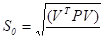
Furthermore, the standard deviation indicated in each calculation is obtained using the following formula:
where:
S0 = Standard deviation
P = Weight matrix
r = Degrees of freedom of the system
The degrees of freedom are calculated by subtracting the number of observation equations (m) minus the number of unknowns (n):
r = m – n
The standard deviation for each of the adjusted values is obtained from the formula:
where:
Sxi = Standard deviation from the adjusted value i
S0 = Total standard deviation of the adjustment
Qxixi = Diagonal element of row i, column i of the covariance matrix
The covariance matrix is calculated using the equation:
where:
Q = Covariance matrix
A = Coefficient matrix
P = Weight matrix
Wolf, P.R. & Ghilani, C.D. (1996). Adjustment computations: statistic and least squares in surveying and GIS.
Brinker, R. C. & Minnick, R. (1995). The Surveying Handbook.